


Plugin Information
| Version | 1.2.1 |
|---|---|
| Author | Dataiku |
| Released | 2021-02 |
| Last updated | 2023-04 |
| License | Apache-2.0 |
| Source code | Github |
| Reporting issues | Github |
⚠️ Starting with DSS version 11 this plugin is considered as “deprecated”, we recommend using the native time series forecasting features.
“Forecasting is required in many situations: deciding whether to build another power generation plant in the next five years requires forecasts of future demand; scheduling staff in a call centre next week requires forecasts of call volumes; stocking an inventory requires forecasts of stock requirements. Forecasts can be required several years in advance (for the case of capital investments), or only a few minutes beforehand (for telecommunication routing). Whatever the circumstances or time horizons involved, forecasting is an important aid to effective and efficient planning.”
— Hyndman, Rob J. and George Athanasopoulos
With this plugin, you will be able to forecast multivariate time series from year to minute frequency with Deep Learning and statistical models. It covers the cycle of model training, evaluation, and prediction, through the two following recipes:
- Train and evaluate forecasting models: Train forecasting models and evaluate them on historical data
- Forecast future values: Use trained forecasting models to predict future values after your historical dataset
Table of contents
How to set up
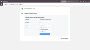
Right after installing the plugin, you will need to build its code environment. If this is the first time you install this plugin, click on Build new environment.
Note that Python version 3.6 or 3.7 is required, with system development tools and Python interpreter headers to build the packages. You can refer to this documentation if you need to install these beforehand.
Warning: if you were previously using the former forecast plugin and now want to use this new forecast plugin instead, you will need to update the existing flows with new recipes.
How to use
In this section, we will use the example of forecasting retail sales across multiple stores and departments. You can find the underlying data and flow on this public gallery project.
1. Train and evaluate forecasting models
Use this recipe to train forecasting models and evaluate them on historical data.
Input
- Historical dataset with time series data (one parsed date column, one or more numerical target columns, and optionally one or more time series identifiers columns)
Output
- Trained model folder to save trained forecasting models
- Performance metrics dataset of forecasting models evaluated on a split of the historical dataset
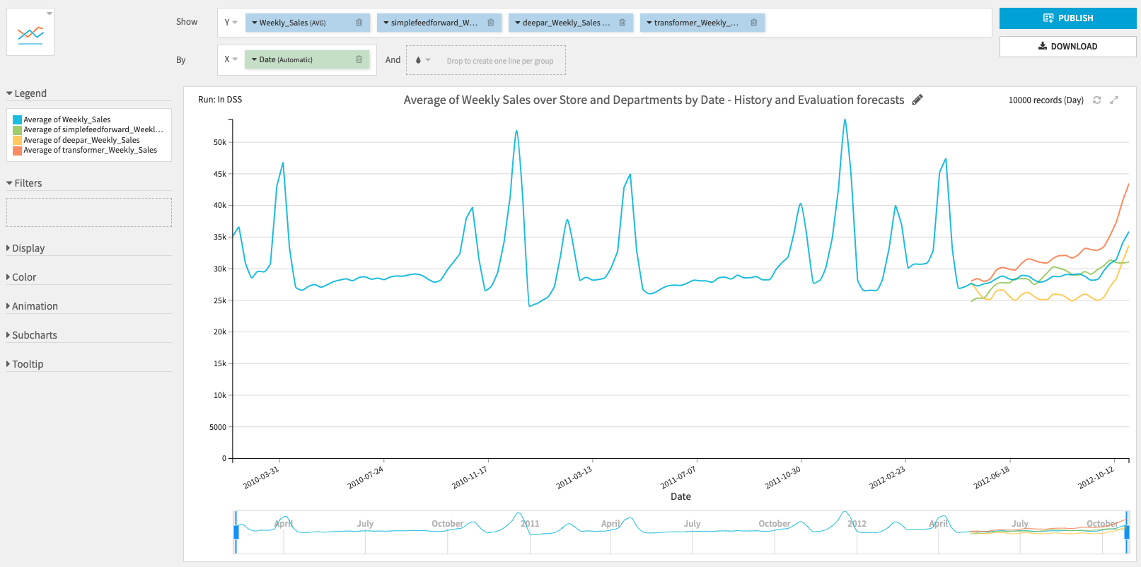
- Evaluation dataset with evaluation forecasts used to compute the performance metrics
- This dataset can be used to build charts and visualize your models’ performance
Settings
Input parameters
- Time column: Column with parsed dates and no missing values
- To parse dates, you can use a Prepare recipe.
- To fill missing values, you can use the Time Series Preparation resampling recipe.
- Frequency of the time column, from year to minute
- For minute and hour frequency, you can select the number of minutes or hours.
- For week frequency, you can select the end-of-week day.
- Target column(s): Time series columns you want to forecast (must be numeric)
- You can select one (univariate forecasting) or multiple columns (multivariate forecasting).
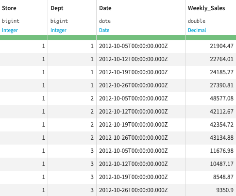
- Long format: Select this option when the dataset contains multiple time series stacked on top of each other
- If selected, you then have to select the columns that identify the multiple time series, with the Time series identifiers parameter.
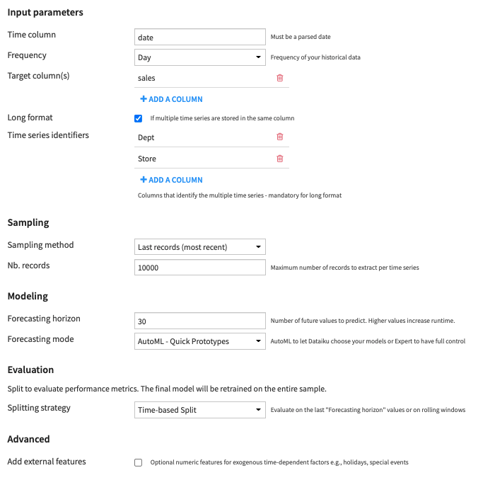
For example, this long format dataset of weekly sales per store and department has Store and Dept as time series identifiers columns
Sampling
- Sampling method: Choose between
- Last records (most recent): To only use the last records of each time series during training (the N most recent data)
- No sampling (whole data): To use all records
- Nb. records: Maximum number of records to extract per time series if Last records was selected
Modeling
- Forecasting horizon: Number of future values to predict
- This number will be reused in the 2. Forecast future values recipe
- Be careful, high values increase training time.
- Forecasting mode: With the following parameter, you can choose to let Dataiku create your models with AutoML modes or have full control over the creation of your models with Expert modes. Check this section to see details on each model.
- You can choose between 4 different forecasting modes:
- AutoML – Quick prototypes (default): Train baseline models quickly
- Statistical models: Trivial identity and Seasonal naive are trained
- Deep Learning models: a FeedForward neural network is trained with 10 epochs of 50 batches with sizes of 32 samples
- AutoML – High performance: Be patient and get even more accurate models
- Statistical models: Trivial identity and Seasonal naive are trained
- Deep Learning models: FeedForward, DeepAR and Transformer are trained with 10 (30 for multivariate) epochs of an automatically adjusted number of batches with sizes of 32 samples
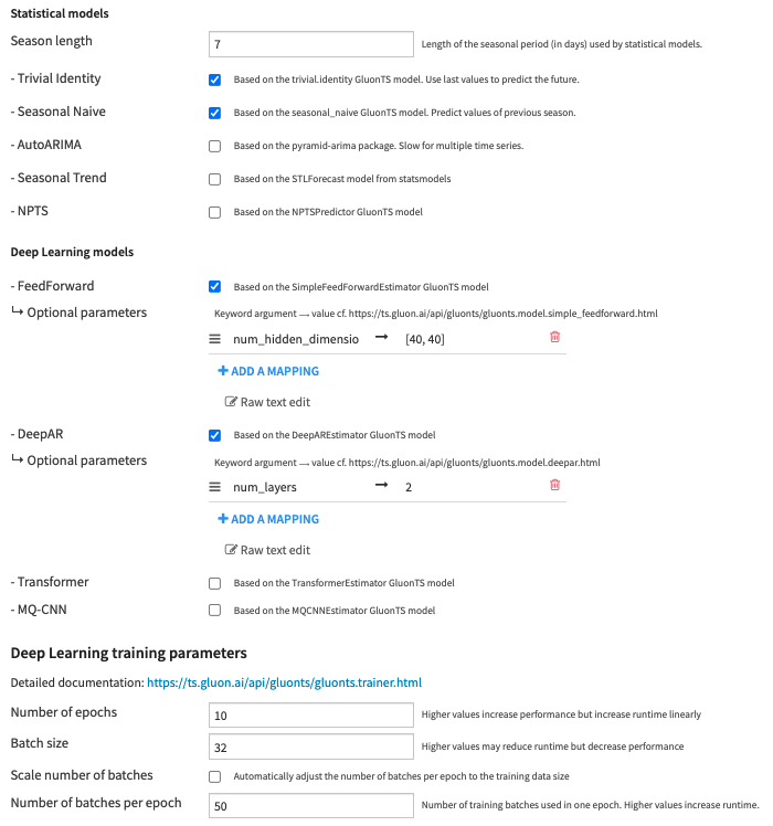
- Expert – Choose algorithms: Choose which models to train, set the seasonality of the statistical models and tune Deep Learning models training parameters
- Season length: Length of the seasonal period (in selected frequency unit) used by statistical models.
- For example, season length is 7 for daily data with a weekly seasonality (season length is 4 for a 6H frequency with a daily seasonality).
- Number of epochs: Number of times the Deep Learning models see the training data.
- Batch size: Number of samples to include in each batch. A sample is a time window of length 2 x forecasting horizon
- Scale number of batches: Automatically adjust the number of batches per epoch to the training data size to statistically cover all the training data in each epoch
- Example: 10 time series of length 10000 will give 209 batches per epoch with a batch size of 32 and a forecasting horizon of 15.
- Number of batches per epoch: Use this to set a fixed number of batches per epoch to ensure the training time does not increase with the dataset size.
- Season length: Length of the seasonal period (in selected frequency unit) used by statistical models.
- Expert – Customize algorithms: Set additional keywords arguments to each algorithm
- AutoML – Quick prototypes (default): Train baseline models quickly
- You can choose between 4 different forecasting modes:
Evaluation
Split to evaluate performance metrics. The final model will be retrained on the entire sample.
- Splitting strategy: Choose between:
- Time-based Split: Evaluate on the last Forecasting horizon values
- Time series cross-validation: Evaluate the forecast predictions on rolling windows
- Models are trained multiple times on expanding rolling windows datasets and metrics computed using the last Forecasting horizon values of each window. The final metrics are averaged over all rolling windows. Two additional parameters must be set:
- Number of rolling windows: Number of splits used in the training set. Higher values increase runtime.
- Cutoff period: Number of time steps between each split. If -1, Horizon / 2 is used.
Advanced
- Add external features: To add numeric features for exogenous time-dependent factors (e.g., holidays, special events).
- External feature columns:
- Be careful that future values of external features will be required to forecast.
- You should only use this parameter for features that you know about in advance, e.g., holidays, special events, promotions.
- If you have features you would like to include in your models but which you do NOT know about in advance, e.g., the weather, we recommend either:
- Including these features as Target columns to forecast
- Using external forecasting data providers, e.g. weather forecasting APIs
- Note that external features are only usable by AutoARIMA, DeepAR, Transformer, and MQ-CNN algorithms.
- External feature columns:
- If you have installed the GPU version of the plugin, please refer to this section on GPU-specific parameters.
2 . Forecast future values
Use this recipe to use trained forecasting models to predict future values after your historical dataset.
Input
- Trained model folder containing models saved by the 1. Train and evaluate forecasting models recipe
- Optional – Dataset to forecast, if not provided, use the training data. The recipe will forecast values after this dataset instead of the data used in training.
- This should contain the exact same column as the training dataset.
- Optional – Dataset with future values of external features only required if you specified external features in the 1. Train and evaluate forecasting models recipe
- This should contain the same time and external features columns (and time series identifiers columns if Long format was activated) as the ones used during training.
Output
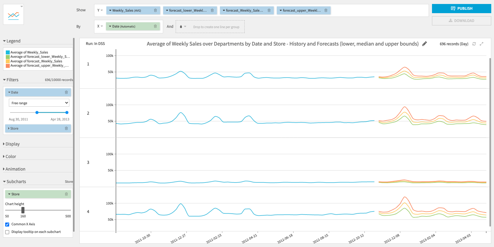
- Forecast dataset with predicted future values and confidence intervals.
- Use it to build charts to visually inspect the forecast results.
Settings
Model Selection
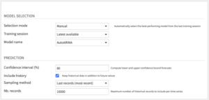
- Selection mode: Choose how to select the model used for prediction.
- Automatic to select the best-performing model from the last training session.
- Performance metric: metric used to retrieve which model has performed best. Lower is better.
- Manual to select yourself a training session and a trained model.
- Training session: UTC Timestamp of the training session from which to retrieve a trained model. Choose “Latest available” to always select the last training session (useful for operationalization).
- Model name: Name of the trained model to retrieve from the selected session. Choose “All models” to forecast values for every trained models.
- Automatic to select the best-performing model from the last training session.
Prediction
- Confidence interval (%): Lower and upper bounds forecasts of the selected confidence interval will be computed.
- Include history: If you want to keep historical data used in training in addition to future values in the output dataset
- Sampling method: if you want to include only the last records of the historical time series (the N most recent data).
- Nb. records: how many records to keep for each time series
Models
Most models are from GluonTS, a time series forecasting Python package that focuses primarily on Deep Learning-based models. We have also added additional statistical models from pmdarima and statsmodels.
Statistical models
- Trivial identity: Baseline model that predicts the same values as the previous forecast horizon values
- Seasonal naive: Automatically finds the season based on the selected frequency and forecast values at the previous season
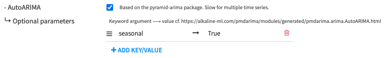
- AutoARIMA: Uses the auto_arima model of the pmdarima package. You can set the season length parameter to be used in ARIMA models in the Expert mode and choose whether to use a seasonal model.
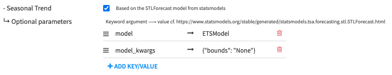
- Seasonal Trend: Model-based forecasting using STL to remove seasonality. The underlying model can be selected among ETSModel and ARIMA in the Expert – Customize algorithms mode and model arguments can be set.
- NPTS: Non-Parametric Time Series Forecaster.
Deep Learning models
Deep Learning models work well with multiple time series of the same nature (either long format or multiple target columns). In multivariate time series forecasting, a single Deep Learning model is trained on all-time series but future values of each time series are predicted using only its own past values.
- FeedForward: Simple Feed-Forward neural network.
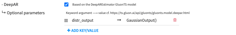
- DeepAR: Auto-regressive neural network.
- Transformer: Transformer neural network.
For FeedForward, DeepAR and Transformer, ‘distr_output’ parameter can be set to StudentTOutput() (default), GaussianOutput() (for real-valued data) or NegativeBinomialOutput() (for positive count data).
- MQ-CNN: Multi-Horizon Quantile Convolutional neural network.
Advanced topics
GPU version
In order to use a GPU to train Deep Learning models, you need to install the GPU version of the plugin that supports a specific CUDA version. The DSS instance server or the container(s) used to execute the plugin recipe must have a GPU setup with the same CUDA version as the plugin. For instance, if your server/container has GPUs with CUDA 10.0 installed, you need to install the “Forecast (GPU – CUDA 100)” plugin.
If you have installed the GPU version of the plugin, additional parameters will be available in the 1. Train and Evaluate recipe, under Advanced. Note that only Deep Learning models can be trained on a GPU. Statistical models are always trained on the CPU.
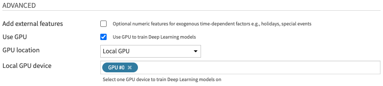
If Use GPU is selected, additional GPU-related parameters can be specified. Else, all models will be trained on the CPU.
- GPU location: Choose between
- Local GPU: If the GPU is on the DSS instance server and the recipe is executed locally
- Container GPU: If the GPU is in a container and the recipe is executed within this container
- You can select a container in the Advanced tab of the recipe > Container configuration
- If the container has multiple GPUs, only the first one will be used
- Local GPU device: Select one GPU device on the DSS instance server
Note that increasing the Batch size (in Deep Learning training parameters) is a good way to make GPU training much faster than on CPU.
Forecasting multiple time series
When forecasting multiple time series, you have two options:
- (Recommended) Activate Long format and add Time series identifiers in Input parameters
- This will train multivariate models that learn from all the time series at the same time.
- Deep Learning models are also able to learn from the links between the different time series, which can greatly enhance the overall forecasting performance.
- In terms of computation, this implies vertical scaling with the number of time series. For instance, if training on 100 time series requires 4GB of RAM, then training on 1000 time series will require 40 GB of RAM.
- Partition your input dataset and train partitioned forecasting models
- This requires your historical dataset to be partitioned. You can follow this tutorial to know how to repartition a non-partitioned dataset.
- Then, instead of activating Long format, you can select which partitions to train/forecast when running the recipes.
- The partition selection can be done manually from the recipe or in the flow.
- Else, you can automate the partition specification in a scenario with project variables.
- This will train one independent forecasting model for the time series within each partition. The model trained for partition A will be used to forecast for partition A, the model for partition B will be used to forecast for partition B, etc. Partitions are run independently so that no data is shared across partitions.
- This behavior can be beneficial if your time series have different patterns and no link with one another. In terms of computation, partition allows horizontal scaling with the number of time series, with a parameter to control concurrency. If you have a Kubernetes cluster, you can distribute each partition in its own pod, and request multiple pods at the same time.
- Note that in this case, if the schema of one of the output datasets is going to change after re-running a recipe (because of changes made to the recipe), you first need to manually drop the dataset schema.
Overall, we strongly recommend the first option before trying the partitioning option. Assuming your training sample can fit in your server/container’s RAM, this option will likely be faster, better in terms of performance, and simpler to implement.
Using forecasting models in production
The recommended workflow to use this forecasting plugin in production is to automate a batch process using a scenario with steps to:
-
- Fetch the latest historical data from your favorite data sources
- Prepare your data, for instance with the Time Series Preparation plugin
- Re-train and evaluate forecasting models on the new data
- Bonus: you can set up a reporting alert related to the latest performance metrics
- Compute the new forecasts with the Forecast future values recipe
- Export the results: write directly to one of your operational systems, send them by email, share them with another Dataiku user, etc.
This batch process can be scheduled to run every weekend, night, hour, or even every 5 minutes. If you have strict time constraints on the overall process duration, we recommend investing in a GPU, as this can greatly accelerate training speed.
Note that for now, the plugin is not meant for real-time production (below 1 minute). If you have a use case that requires real-time, please contact us at [email protected].