


Before using time series data for analysis or forecasting, it is often necessary to perform one or more preparation steps on the data.
For example, given time series data with missing or irregular timestamps, you may consider performing preparation steps such as resampling and interpolation. You may also want to perform smoothing, extrema extraction, segmentation on the data or time series decomposition.
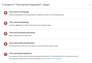
The time series preparation plugin provides visual recipes for performing resampling, windowing operations, interval extraction, extrema extraction and decomposition on time series data.
Components of the Time Series Preparation Plugin
This plugin is fully supported by Dataiku. For usage details, see the reference documentation. To learn more about the plugin, check out the dedicated online course.
Table of contents
How to set up
Right after installing the plugin, you will need to build its code environment. If this is the first time you install this plugin, click on Build new environment.
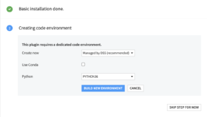
Note that for the plugin version 2 or higher, Python version 3.6 is required with system development tools and Python interpreter headers to build the packages. You can refer to this documentation if you need to install these beforehand.
Warning: if you were previously using the plugin on version 1.3 or older with a python 2 environment and are now upgrading the plugin to version 2.0 or higher, you will need to delete the python environment and create a new one with Python 3.6.
How to use
All the recipes of the plugin can be used on a dataset that contains time series. The date column must be parsed. Time series can be stored in wide or long format.
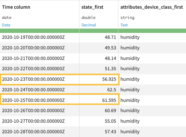
Time Series resampling
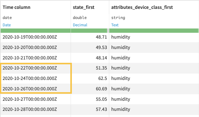
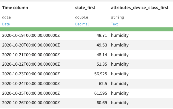
The resampling recipe transforms time series data occurring in irregular time intervals into equispaced data. The recipe is also useful for transforming equispaced data from one frequency level to another (for example, minutes to hours).
This recipe resamples all numerical columns (type int or float) and imputes categorical columns (type object or bool) in your data.
Input
- A dataset that consists of n-dimensional time series in wide or long format.
Output
- A dataset consisting of equispaced time series, and having the same number of columns as the input data.
Settings
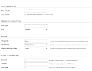
Input parameters
- Time column: Name of the column that contains the timestamps. Note that the timestamp column must be parsed, and duplicate timestamps cannot exist for a given time series.
- Long format: Select this option when the dataset contains multiple time series stacked on top of each other
- If selected, you then have to select the columns that identify the multiple time series, with the Time series identifiers parameter.
Resampling parameters
- Time step: Number of steps between timestamps of the resampled (output) data, specified as a numerical value
- Unit: Unit of the time step used for resampling.
Methods
- Interpolate: Method used for inferring missing values for timestamps, where the missing values do not begin or end the time series. More details about the available methods in the documentation.
- Extrapolate: Method used for prolonging time series that stop earlier than others or start later than others. Extrapolation infers time series values that are located before the first available value or after the last available value. More details about the available methods in the documentation.
- Impute categorical data: Method used to fill in categorical values during interpolation and extrapolation. More details about the available methods in the documentation.
Advanced parameters
- Clip start: Number of time steps to remove from the beginning of the time series, specified as a numerical value of the unit parameter.
- Clip end: Number of time steps to remove from the end of the time series, specified as a numerical value of the unit parameter.
- Shift value: Amount by which to shift (or offset) all timestamps, specified as a positive or negative numerical value of the unit parameter.
Time Series windowing
For high frequency or noisy time series data, observing the variations between successive observations may not always provide insightful information. In such cases, it can be useful to filter or compute aggregations over a rolling window of timestamps.
The windowing recipe allows you to perform analytics functions over successive periods in equispaced time series data. This recipe works on all numerical columns (type int or float) in your data.
Input
- A dataset that consists of equispaced n-dimensional time series in wide or long format. To fill missing values, you can use the Resampling recipe.
Output
- A dataset consisting of equispaced time series, with additional columns for each aggregation.
Settings
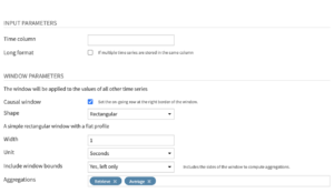
Input parameters
- Time column: Name of the column that contains the timestamps. Note that the timestamp column must be parsed, and duplicate timestamps cannot exist for a given time series.
- Long format: Select this option when the dataset contains multiple time series stacked on top of each other
- If selected, you then have to select the columns that identify the multiple time series, with the Time series identifiers parameter.
Window parameters
- Causal window: Option to use a causal window, that is, a window which contains only past (and optionally, present) observations. The current row in the data will be at the right border of the window. If you de-select this option, Dataiku DSS uses a bilateral window, that is, a window which places the current row at its center.
- Shape: Window shape applied to the Sum and Average operations. More details about the available options in the documentation.
- Width: Width of the window, specified as a numerical value (int or float). The window width cannot be smaller than the frequency of the time series.
- Unit: Unit of the window width.
- Include window bounds: Edges of the window to include when computing aggregations. This parameter is active only when you use a causal window.
- Aggregations: Operations to perform on a window of time series data. More details about the available options in the documentation.
Time series extrema extraction
Time series extrema refers to the minimum and maximum values in time series data. It can be useful to compute aggregates of a time series around extrema values to understand trends around those values.
The extrema extraction recipe allows you to extract aggregates of time series values around a global extremum (global maximum or global minimum).
Using this recipe, you can find a global extremum in one dimension of a time series and perform windowing functions around the timestamp of the extremum on all dimensions.
Input
- A dataset that consists of equispaced n-dimensional time series in wide or long format. To fill missing values, you can use the Resampling recipe. If input data is in the long format, then the recipe will find the extremum of each time series in the column on which you operate.
Output
- A dataset consisting of the results of extrema extraction, one row for each time series. Each row contains the timestamp of the extremum and the computed aggregations for a window of data around the extremum.
Settings
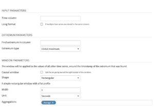
Input parameters
- Time column: Name of the column that contains the timestamps. Note that the timestamp column must be parsed, and duplicate timestamps cannot exist for a given time series.
- Long format: Select this option when the dataset contains multiple time series stacked on top of each other
- If selected, you then have to select the columns that identify the multiple time series, with the Time series identifiers parameter.
Extrema parameters
- Find extremum in column: Name of column from which to extract the extremum value.
- Extremum type: Type of extremum to find, specified as “Global minimum” or “Global maximum”.
Window parameters
- Causal window: Option to use a causal window, that is, a window which contains only past (and optionally, present) observations. The timestamp for the extremum point will be at the right border of the window. If you de-select this option, Dataiku DSS uses a bilateral window, that is, a window which places the timestamp for the extremum point at its center.
- Shape: Window shape applied to the Sum and Average operations. More details about the available options in the documentation.
- Width: Width of the window, specified as a numerical value (int or float). The window width cannot be smaller than the frequency of the time series.
- Unit: Unit of the window width.
- Include window bounds: Edges of the window to include when computing aggregations. This parameter is active only when you use a causal window.
- Aggregations: Operations to perform on a window of time series data. More details about the available options in the documentation.
Time series interval extraction
It is sometimes useful to identify periods when time series values are within a given range. For example, a sensor reporting time series measurements may record values that fall outside an acceptable range, thus making it necessary to extract segments of the data.
The interval extraction recipe allows you to find segments of the time series where values of a column are inside an interval, while allowing small deviations. See Algorithms for more information. This recipe works on all numerical columns (int or float) in your time series data.
Input
- A dataset that consists of equispaced n-dimensional time series in wide or long format. To fill missing values, you can use the Resampling recipe. If input data is in the long format, then the recipe will separately extract the intervals of each time series that is in a column.
Output
- A dataset consisting of equispaced and discontinuous time series. Each interval in the output data will have an id (“interval_id”).
Settings
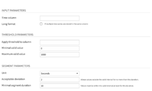
Input parameters
- Time column: Name of the column that contains the timestamps. Note that the timestamp column must be parsed, and duplicate timestamps cannot exist for a given time series.
- Long format: Select this option when the dataset contains multiple time series stacked on top of each other
- If selected, you then have to select the columns that identify the multiple time series, with the Time series identifiers parameter.
Threshold parameters
- Apply threshold to column: Name of the column to which the recipe applies the threshold parameters.
- Minimal valid value: Minimum acceptable value in the time series interval, specified as a numerical value (int or float).
- Maximum valid value: Maximum acceptable value in the time series interval, specified as a numerical value (int or float).
The maximum valid value and the minimal valid value form the range of acceptable values.
Segment parameters
- Unit: Unit of the acceptable deviation and the minimal segment duration
- Acceptable deviation: Maximum duration of the specified unit, for which values within a valid time segment can deviate from the range of acceptable values. For example, if you specify 400 – 600 as a range of acceptable values, and an acceptable deviation of 30 seconds, then the recipe can return a valid time segment that includes values outside the specified range, provided that those values last for a time duration that is less than 30 seconds.
- Minimal segment duration: The minimum duration for a time segment to be valid, specified as a numerical value of the unit parameter. For example, you can specify 400 – 600 as a range of acceptable values, and a minimal segment duration of 3 minutes. If all the values in a time segment are between 400 and 600 (or satisfy the acceptable deviation), but the segment lasts less than 3 minutes, then the time segment would be invalid.
Time series decomposition
Trend/seasonal decomposition is useful to understand, clean, and leverage your time series data. Not only is it necessary to retrieve seasonally-adjusted data, but it is also relevant for anomaly detection. This recipe decomposes the numerical columns of your time series into three components: trend, seasonality and residuals.
The recipe relies on STL, seasonal and trend decomposition using Loess. For more information, see Statsmodel’s documentation
Input
- A dataset that consists of equispaced n-dimensional time series in wide or long format. To fill missing values, you can use the Resampling recipe.
Output
- The output dataset is the same as the input dataset with one additional column for each decomposition component.
Settings
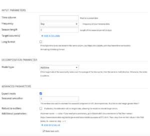
Input parameters
- Time column: Name of the column that contains the timestamps. Note that the timestamp column must be parsed, and duplicate timestamps cannot exist for a given time series.
- Frequency: Frequency of the time column, from year to minute.
- Season length: Length of the seasonal period in selected frequency unit.
- Target column: Time series columns that you want to decompose. It must be numeric (int or float). You can select one or multiple columns.
- Long format: Select this option when the dataset contains multiple time series stacked on top of each other
- If selected, you then have to select the columns that identify the multiple time series, with the Time series identifiers parameter.
Decomposition parameter
- Model type: The decomposition model of your time series. It may be :
- Additive : Time series = trend + seasonality + residuals
- Multiplicative : Time series = trend × seasonality × residuals
If the magnitude of the seasonality varies with the mean of the time series, then the series is multiplicative. Otherwise, the series is additive.
Advanced parameters
If the expert mode is selected, you will be able to choose the value of the following parameters:
- Seasonal smoother: Number of consecutive timesteps (years, weeks..) used in estimating each value in the seasonal component. It controls how rapidly the seasonal component can change.
- Robust to outliers: If selected, the estimation will re-weight data, allowing the model to tolerate larger errors.
- Additional parameters: This map parameter enables you to add any other parameter of the statsmodel STL function. To add a parameter, click on “ADD KEY/VALUE”, then enter the parameter name as the ‘key’, and the parameter value as the ‘value’.