Plugin information
| Version | 1.1.2 |
|---|---|
| Author | Dataiku (Agathe Guillemot and Simona Maggio) |
| Released | 2021-12-24 |
| Last updated | 2025-03-13 |
| License | Apache Software License |
| Source code | Github |
| Reporting issues | Github |
Description
Machine learning models are often trained and evaluated on carefully curated datasets for optimal results, however their performance on real-world data is rarely similar due to disparities in the data quality and distribution.
It can therefore be useful to simulate some of the information degradation that is likely to occur, and evaluate whether the model performs adequately.
The plugin lets you randomly apply distribution shifts & feature corruptions, and check the impact on the model’s performance.
Setup
Right after installing the plugin, you will need to build its code environment. Note that this code environment is in Python version 3.6 or 3.7. It will be used by the visual recipe only: since v1.0.4, the model view will use the code env with which the model was trained.
Deep learning models are not supported.
How to use
Model view: Stress test center
The Stress test center model view offers an interface to configure and run stress tests corresponding to the data changes you expect at deployment time.
When you run the tests, the webapp extracts a sample of the model’s test set, hereafter referred to as the control dataset. For each stress test it creates a copy of this control dataset with data variations. The control dataset and the altered datasets are then preprocessed and scored with the model.
You can then evaluate how your model performs for each stress test.
Reminder: Since Dataiku DSS v9.0.2, model views can also be used in Lab models and in “Saved model report” tiles on dashboards.
Settings
You select and configure the different model stress tests on the left panel of the model view.
General settings
This section contains settings common to all the stress tests, namely:
– The evaluation metric to assess the changes in the model’s performance
– Parameters to sample the model’s test set (the ratio of rows from the model’s test set to use for all the stress tests, the random seed)
Target distribution shift
This section contains one test, available for classification tasks only.
Shift target distribution
This stress test resamples the test set to match the desired distribution for the target.
Target class > Proportion: For each of the model’s classes, you can map a desired proportion of rows belonging to that class to appear in the dataset. The dataset size remains the same, meaning depending on the initial distribution, some rows will be discarded whereas others will be oversampled.
Note that you can provide an incomplete distribution (i.e. with desired proportions on some classes but not all): the proportions will be redistributed equally amongst the remaining classes.
Feature distribution shift
This section contains one test, available for categorical features.
Shift feature distribution
This stress test resamples the test set to match the desired distribution for a selected categorical feature.
Feature category > Proportion: For each of the model’s categories, you can map a desired proportion of rows belonging to that category to appear in the dataset. The dataset size remains the same, meaning depending on the initial distribution, some rows will be discarded whereas others will be oversampled.
Note that here again, you can provide an incomplete distribution (i.e. with desired proportions on some categories but not all): the proportions will be redistributed equally amongst the remaining categories.
Feature corruptions
Each of these independent tests corrupts one or several features across randomly sampled rows. The stress tests are restricted to features of certain variable types.
This section contains two tests.
Insert missing values (available for variable types Numerical, Categorical, Text, Vector)
This stress test removes feature values on randomly selected rows.
Corrupted features: Set one or several features where the values will be removed.
Ratio of corrupted samples: Set the ratio of samples from the control dataset where the values will be removed. The values will be removed for all the selected features simultaneously.
Multiply by a coefficient (available for variable type Numerical)
This stress test multiplies numerical features by a coefficient on randomly selected rows.
Corrupted features: Set one or several numerical features that will be multiplied by a fixed coefficient.
Coefficient: Set the multiplying factor that will be applied on the selected features.
Ratio of corrupted samples: Set the ratio of samples from the control dataset where the values will be multiplied. The values will be multiplied for all the selected features simultaneously.
Results
Metrics
For each test, the resilience of your model is measured via several metrics that compare the model’s performance before and after the data changes and corruptions. The metrics are grouped by test types (Target distribution shift, Feature distribution shift, Feature corruptions).
Performance variation: the difference in performance before and after applying the stress test. The evaluation metric used is the one selected in the General settings section.
The performance metric before and after are also displayed for contextualisation.
Worst subpopulation performance (for Feature distribution shift only): the worst-case performance across all the categories of a categorical feature. The evaluation metric used is the one selected in the General settings section.
Note that both these metrics leverage the evaluation metric selected in the settings. In the case where the computation of the evaluation metric would have failed (for instance, when attempting to compute recall when there are no true positive nor false negative values), accuracy is used instead.
Corruption resilience (for Feature corruptions only):
- For classification, it is the ratio of rows where the predicted value is the same before and after the corruption.
- For regression, it is the ratio of rows where the error between the predicted and true values is not greater after the corruption.
It is at least equal to the proportion of non-corrupted samples.
Critical samples (for Feature corruptions only)
The critical samples are up to five records identified as being most vulnerable to the feature corruptions. They are displayed as cards like this one:
The critical sample card header shows either the average true class probability ± standard deviation (for classification), or the average predicted value ± standard deviation (for regression). The average and standard deviation are computed from the values on the control dataset and its altered versions generated by the stress tests.
The feature values showcased in the card are the ones from the control dataset (i.e. the ones from the model’s test set).
Recipe: Corruption recipe
Input: a single dataset
Output: a single dataset
The recipe applies one of the feature corruptions on an input dataset. The settings are the same as in the model view.
The output dataset can then for instance be used with an evaluation recipe:


