


Example data drift analysis in Dataiku DSS.
Plugin information
| Version | 3.1.6 |
|---|---|
| Author | Dataiku (Léo Dreyfus-Schmidt & Du Phan & Thibault Desfontaines) |
| Released | 2019-11-11 |
| Last updated | 2022-08-10 |
| License | MIT License |
| Source code | Github |
| Reporting issues | Github |
⚠️ Starting with DSS version 10, this plugin is considered as “Deprecated” and will be maintained only to fix critical issues. We recommend using the native feature Model Evaluation Store.
Description
Monitoring ML models in production is often a tedious task. You can apply a simply retraining strategy based on monitoring the model’s performance: if your AUC drops by a given percentage, retrain. Although accurate, this approach requires to obtain the ground truth for your predictions, which is not always fast, and certainly not “real time”.
Instead of waiting for the ground truth, we propose to look at the recent data the model has had to score, and statistically compare it with the data on which the model was evaluated in the training phase. If these datasets are too different, the model may need to be retrained.
Installation Notes
The plugin can be installed from the Plugin Store or via the zip download (see above).
The plugin uses a custom code environment. This one needs to have the same python version as the one used in the visual ML part in order to load the deployed model.
The plugin supports python classification and regression models.
Principle
To detect drift between the original test dataset used by the model and the new data, we stack the two datasets and train a RandomForest (RF) classifier that aims at predicting data’s origin. This is called the domain classifier in the literature.
To have a balanced train set for this RF model, we take the first n samples from the original dataset and the new one, where n is the size of the smallest dataset.
If this model is successful in its task, it implies that data used at training time and new data can be distinguished, we can then say that the new data has drifted.
How to use
Data drift model view
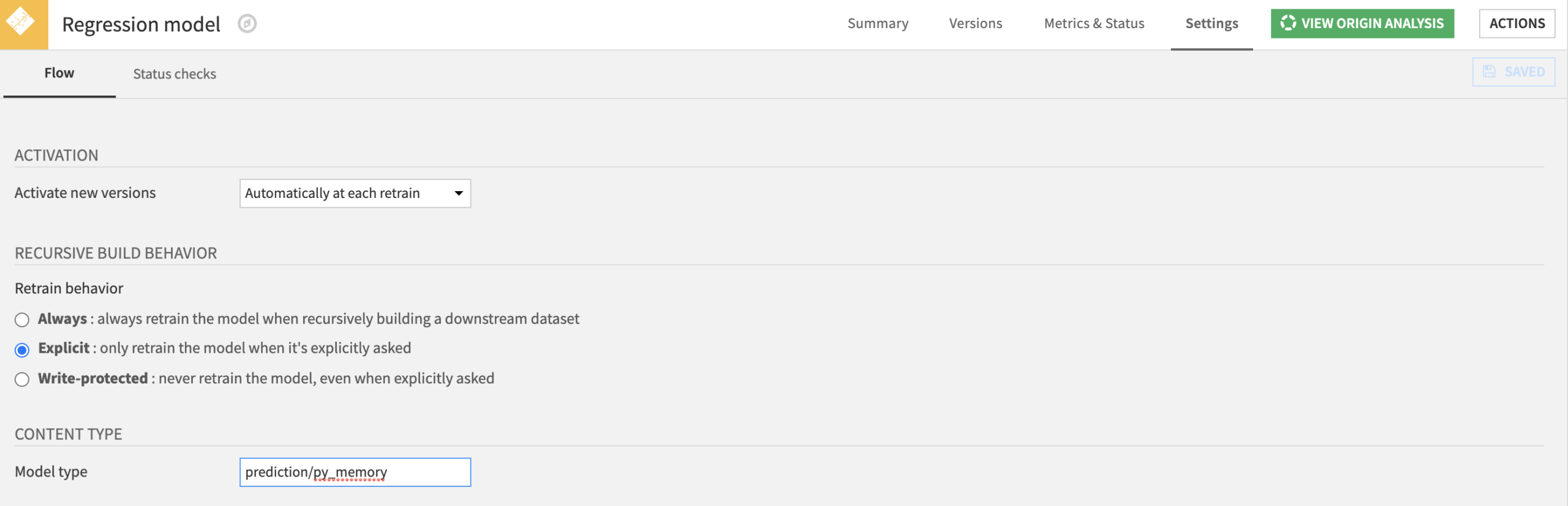
Reminder: A model view is an additional way to visualise information about a model, model views appear in a deployed model’s version page. This is a new feature in DSS v6, if your models are deployed before v6 and you don’t see the “Views” tab, please go back to the saved model screen -> Settings and fill the Model type field with “prediction/py_memory“.
Inputs
- A deployed model that we want to monitor.
- A dataset containing new data the model is exposed to.
Metrics and Charts
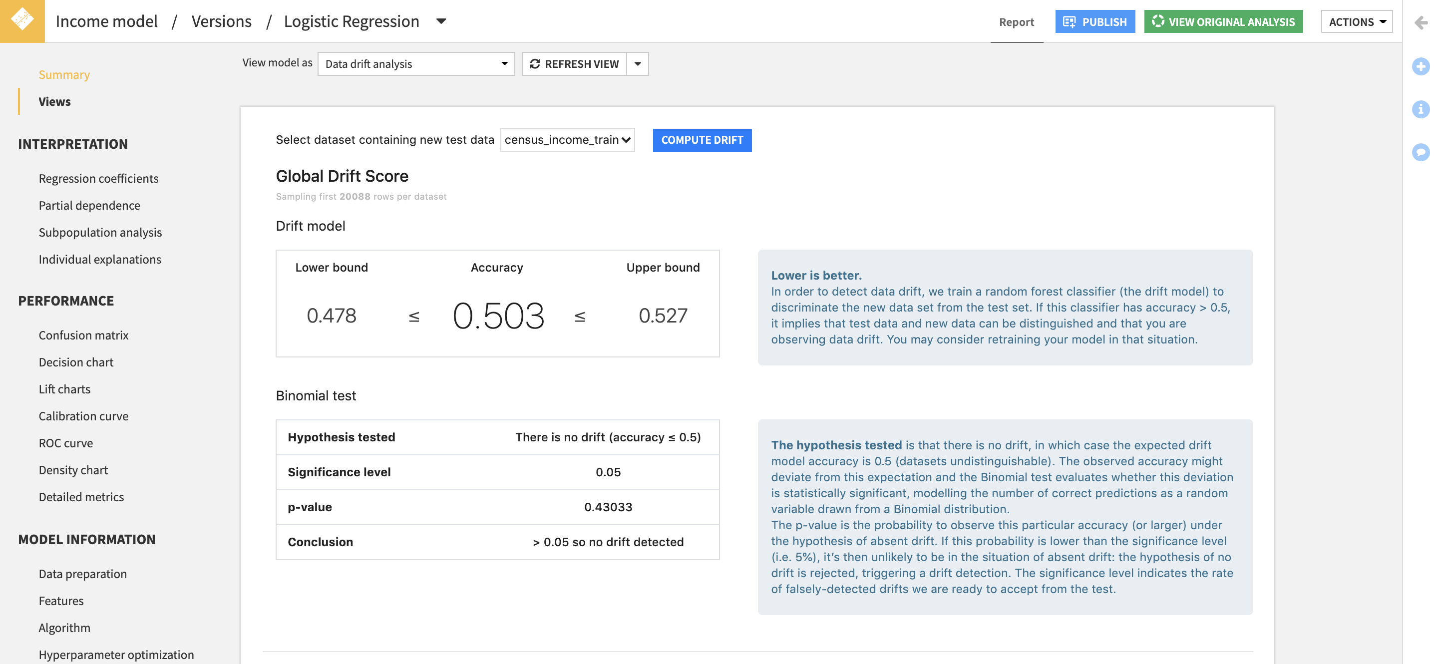
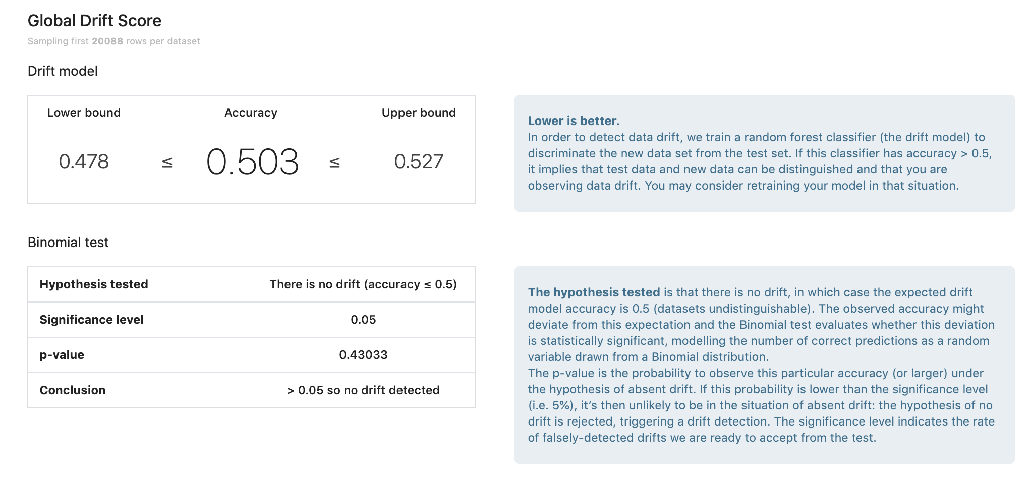 We apply a binomial test on the accuracy of the domain classifier. The null hypothesis being there is no drift.
There are two informations that are computed:
- The p-value which gives the probability of having at least the computed accuracy under the null hypothesis.
- The confidence interval of the computed accuracy given the sample size.
The confidence interval gives us an indice about the reliability of the drift score. If we get an accuracy score of 0.65 ± 0.2, the score is not very reliable as it overlaps with 0.5, which means no drift.
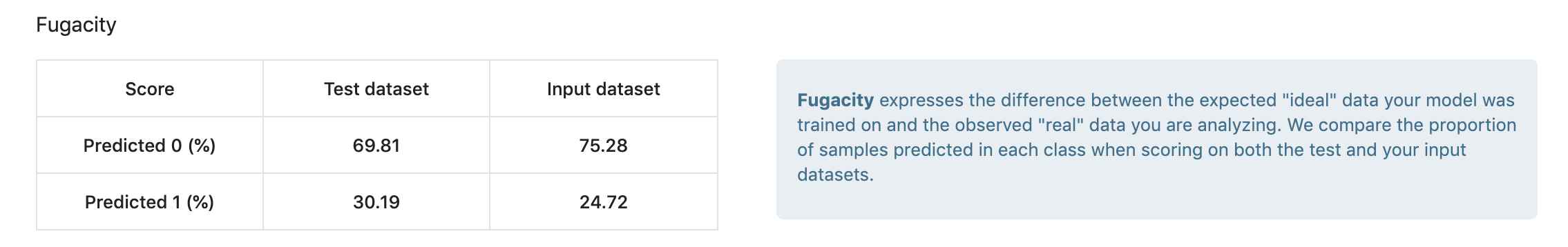
Fugacity measures the difference between the expected “ideal” data your model was trained on and the observed “real” data you are analysing. We compare the proportion of samples predicted in each class when scoring on both the test and your input datasets.
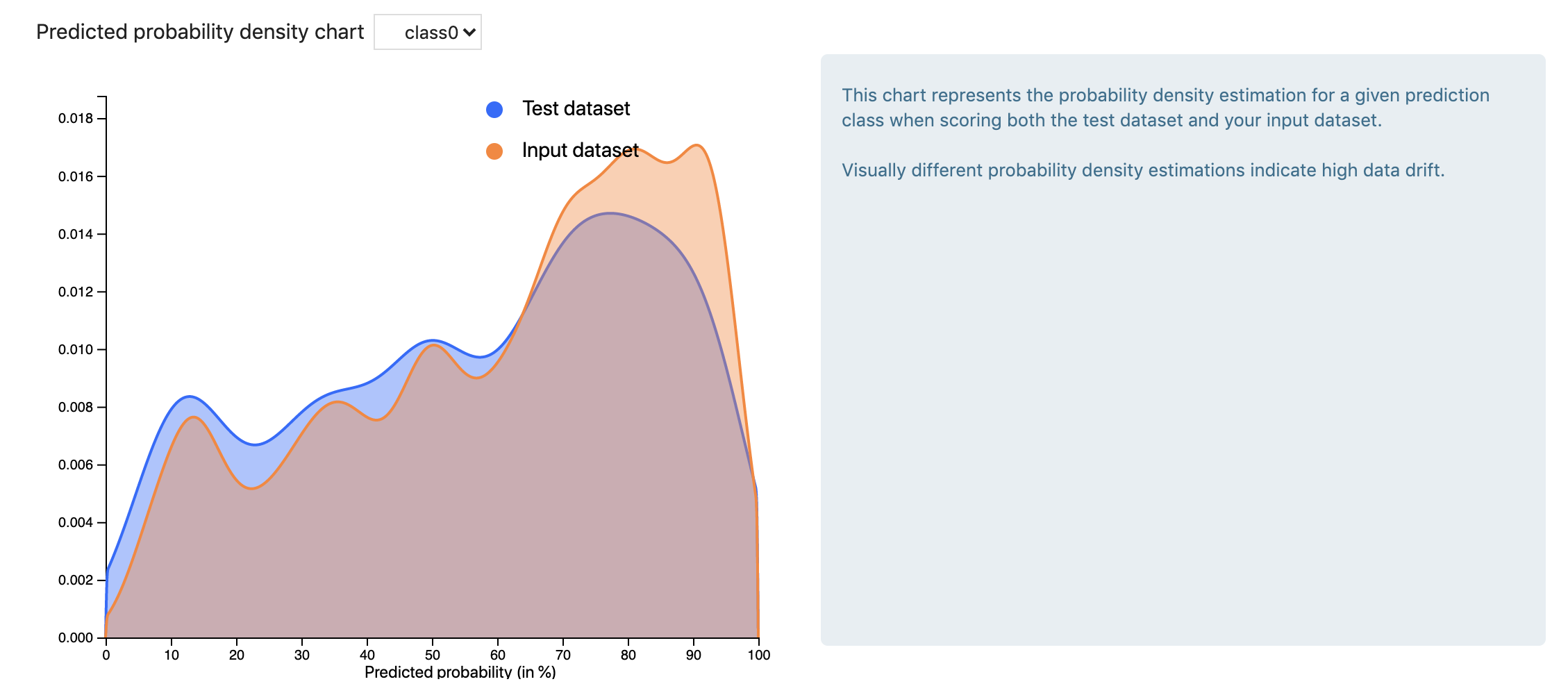
This chart represents the probability density estimation for a given prediction class when scoring both the test dataset and your input dataset.
Visually different probability density estimations indicate high data drift. The inverse is not true, as we can have a high drift score but a similar predicted probability density estimation. One such situation is when we have high drift of a feature that is not important in the original model.
Feature importance comparison
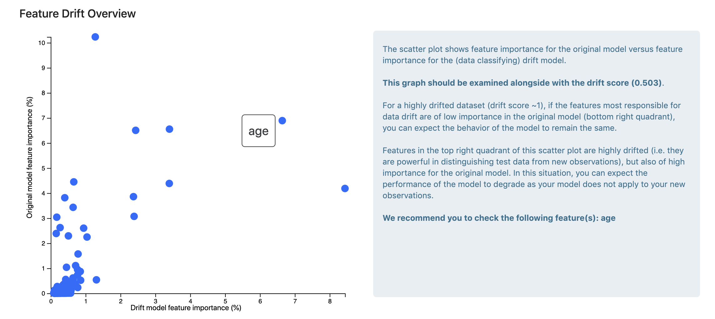
The scatter plot shows feature importance for the original model versus feature importance for the (data classifying) drift model.
This graph should be examined alongside with the drift score. For a highly drifted dataset (drift score close to 1), if the features most responsible for data drift are of low importance in the original model (bottom right quadrant), you can expect the behavior of the model to remain the same.
Features in the top right quadrant of this scatter plot are highly drifted (i.e. they are powerful in distinguishing test data from new observations), but also of high importance for the original model. In this situation, you can expect the performance of the model to degrade as your model does not apply to your new observations.
Note: This chart only appears when the drift is significant (its score is >= 0.1), otherwise it can be misleading (you can always retrieve the most important features of a RF model even when the model is bad).
Recipe: compute input drift of a deployed model
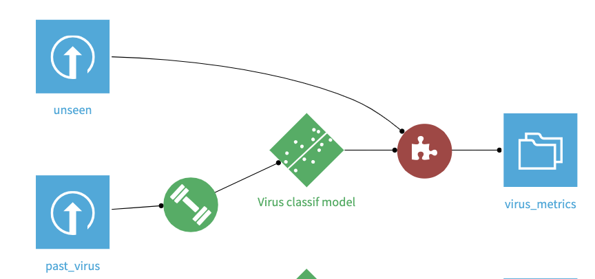
Inputs
This recipe replicates the behaviour of the model view above. It takes as input:
- A deployed model
- A new dataset
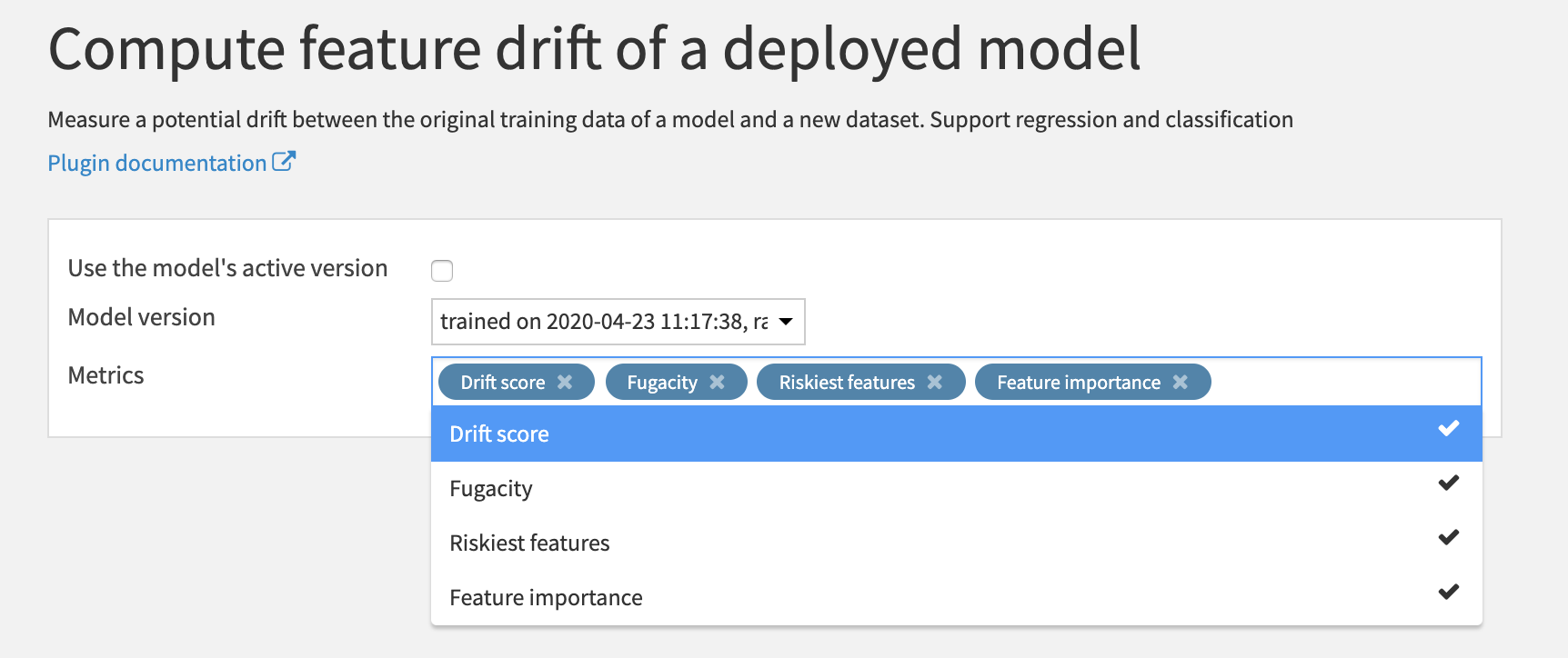
Output
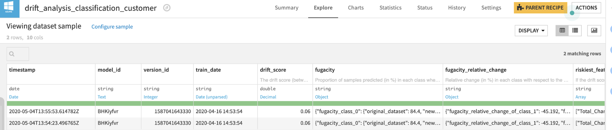
It provides 4 types of information:
Drift score
Fugacity
Fugacity raw value:
- For classification model: proportion of samples predicted (in %) in each class when scoring on both the original test and the new input dataset.
- For regression model: proportion of samples predicted (in %) in each decile when scoring on both the original test and the new input dataset.
Fugacity relative change:
For classification model:
- Relative change (in %) in each class with respect to the original fugacity value.
- Formula: 100*(new_fugacity – original_fugacity)/original_fugacity
For regression model:
- Relative change (in %) in each decile with respect to the raw fugacity value.
- Formula: 100*(new_fugacity – original_fugacity)/original_fugacity
Riskiest features
- List of features that are in the top 40% of both the list of most drifted features AND the most important feature in the original model.
- Note: this information should only be used when drift score is medium/high (above 0.1), for a low drift the features were not really drifted, thus the info is not significant.
Feature importance
- Most drifted features: like the riskiest features part, this information should be interpreted alongside the drift score. With a low drift score, it is not important. For a medium/high drift score (above 0.1), the drift degree of each feature is significant and thus the information is interesting.
- Most important features in the original model.
Recipe: compute drift between two datasets
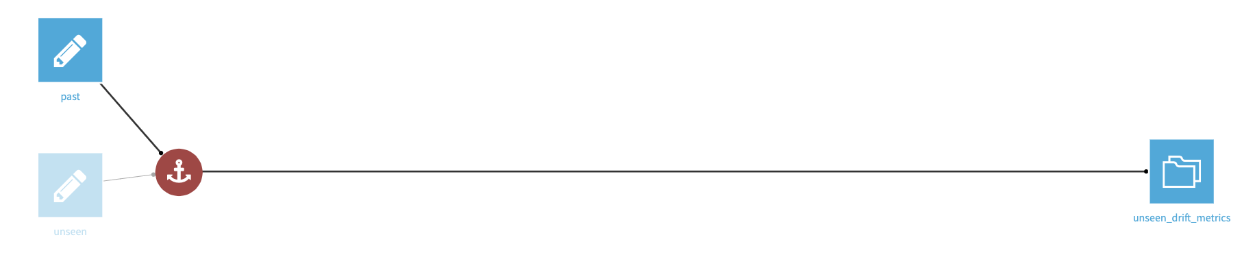
This recipe allows users to compare data drift between two datasets sharing the same schema.
This recipe aims at people who mostly build KPI from data, each day when new data comes in they want to have a tool to assess whether or not the new data is “different”.
It provides 2 types of information:
- Drift score
- Most drifted features
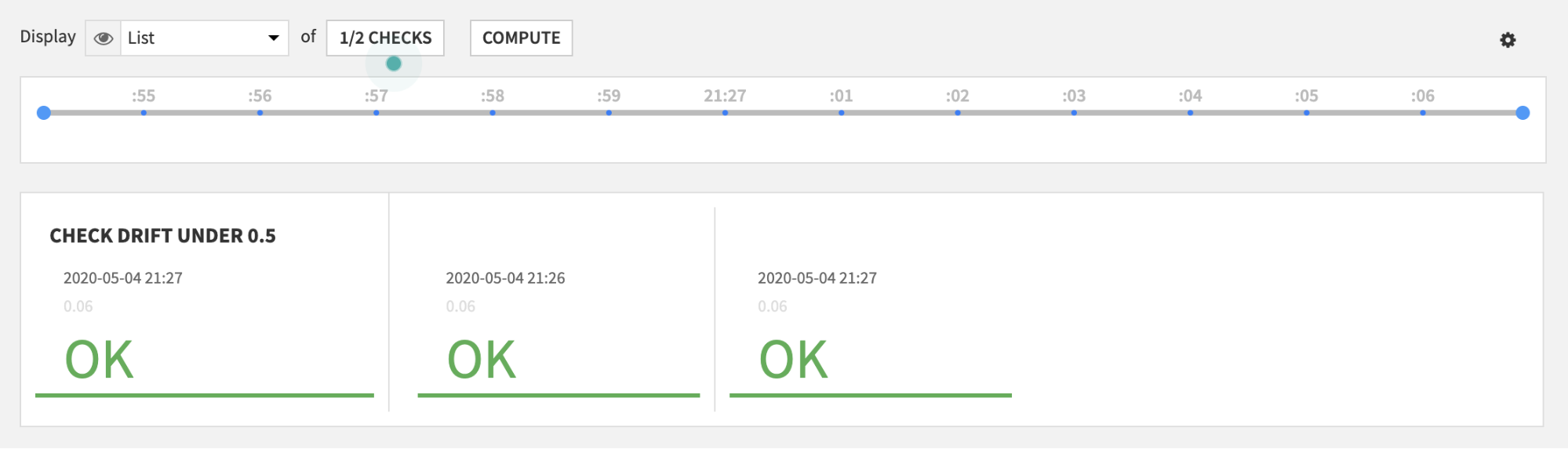
Custom metric: retrieve most recent drift score
This component must be used alongside the above recipes. Once users have created a drift recipe, they can set the recipe to “append” mode (in the Input/Output tab) to get the daily drift score for example and then use this custom metric to retrieve the most recent drift score.
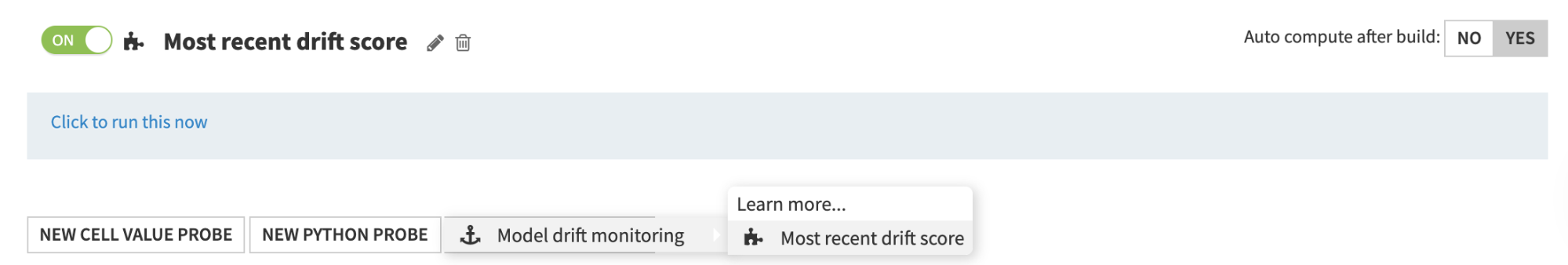
From there, users can create a custom check with their own threshold and put these in a scenario for drift monitoring.