


Plugin information
| Version | 1.1.1 |
|---|---|
| Author | Dataiku (David Behar, Matthew Galloway, Nicolas Vallée) |
| Released | 2022-03-03 |
| Last updated | 2024-02-27 |
| License | Software License |
| Source Code | Github |
| Reporting issues | Github |
Description
Generalized Linear Models (GLMs) are a generalization of the Ordinary Linear Regression where:
- The distribution of the response variable can be chosen from any exponential distribution (not only a gaussian distribution).
- The relationship between the linear model and the response variable can be chosen from any link function (not only the identity function).
These models allow flexibility on the dependency between the regressors and the response and are widely used in the Insurance industry to answer specific modelization needs. The GLM implementation comes from glum package. Regression Splines rely on patsy.
How to set up
The plugin is available through the plugin store. When downloading the plugin, the user is prompted to create a code environment, it should be on python 3.8 or 3.9. The plugin components are listed on the plugin page and can then be used in the projects of the instance. This plugin requires Dataiku V12+.
To use the Generalized Linear Model Regression and Classification algorithms in the visual ML, a specific code environment needs to be selected in the runtime environment. An exception is raised if not. This code environment needs the required visual ML packages as well as the glum package. Otherwise, the user should go through the following steps:
- Create a python 3.8+ code environment in Administration > Code Envs > New Env.
- Go to Packages to install.
- Click on Add set of packages.
- Add the Visual Machine Learning packages.
- Add the glum package: glum==2.6.0
- Click on Save and Update.
- Go back to the Runtime Environment
- Select the environment that has been created.
How to use
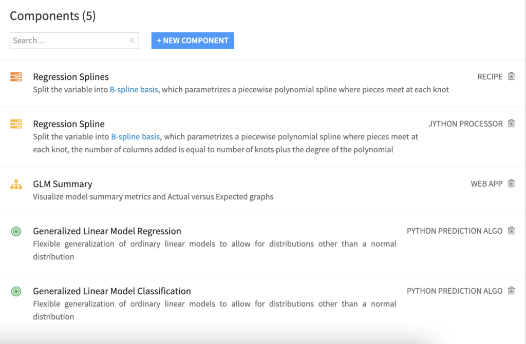
The plugin contains 5 components to enable GLM fitting. The first two are custom models: one for regression and one for binary classification. A custom view is available in the visual ML to visualize metrics specific to GLMs and Actual Expected graphs. Finally, Regression Splines feature engineering capabilities are implemented both as a custom recipe and as a Prepare step.
Generalized Linear Model: Regression
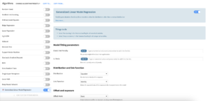
In the visual ML, when selecting a Prediction type, Generalized Linear Models become available in algorithms. The user needs to activate the algorithm and then configure it by inputting the parameters:
- Elastic Net Penalty: constant that multiplies the elastic net penalty terms. For unregularized fitting, set the value to 0.
- L1 ratio: specify what ratio to assign to an L1 vs L2 penalty.
- Distribution: The distribution of the response variable, to be chosen from the list of available distributions (Binomial, Gamma, Gaussian, Inverse Gaussian, Poisson, Negative Binomial, Tweedie). Some of these distributions require additional parametrization that will appear on the screen if needed.
- Function: The function linking the linear regression to the response. The available functions depend on the distribution choice. Some of these functions require additional parametrization that will appear on the screen if needed.
- Mode: The user can either choose not to add offsets or exposures, or to add some. To add exposures columns, the link function must be the log function.
- Training Dataset: When selecting to add offsets or exposures, the user must input the training dataset, which should be associated with the analysis.
- Offset Columns: The names of the offset columns. The offset variables are added to the linear regression (which consists of adding variables with fixed coefficients with value 1).
- Exposure Columns: The names of the exposure columns. The exposure variables are treated exactly like the offset variables but the log function is applied. This is only available when selecting a log function.
Generalized Linear Model: Binary Classification
When the user selects binary classification, the Generalized Linear Model is also added. It contains the same parametrization as the regression. The natural choice for GLM Binary Classification is the Binomial distribution with the logit function, also called logistic regression.
Generalized Linear Model: Summary View
A custom view is available in the part of the visual ML. It can be accessed for a saved model or for analysis, but is only working for GLMs. This view compiles metrics specific to GLMs and Actual Expected graphs.
Metrics
The metrics computed by glum are outputted:
- Bayesian Information Criterion (BIC): This metric takes into account the likelihood of the fitted model with the data, the number of features, and the number of data points. When the number of features increases, the likelihood should increase also because should fit the data better, BIC strikes the balance between both. Lower values of BIC are preferred to prevent overfitting.
- Akaike Information Criterion (AIC): This metric works similarly to BIC but does not take into account the number of data points. Lower values of AIC are also preferred.
- Deviance: This metric is a goodness-of-fit statistic, it computes the difference between the saturated model likelihood and the fitted model likelihood. The saturated model is the perfect fit model that fits a set of parameters for each data point. Deviance thus represents how much the fitted model differs from the perfect fit model.
Actual versus Expected Graphs
Actual versus Expected graphs give a visual representation of the fit with the data. They each compare model responses with actual responses in different ways. The user selects the variable of interest among the columns from the training dataset, excluding the target, whether they were used in the training or not. The variable of interest is binned in 20 bins maximum when it is numerical, grey bars represent the weights of each bin in the dataset.
- The Base Graph: To compute the base response, the features other than the variable of interest are set to their base value. The base value is defined as the mode of the distribution of the feature (when binned if is numerical). For each bin, the base predictions are weighted with the predefined weights. Thereby, the shows the pure effect of the feature on the response. When selecting a variable that is not included in the model, it displays a straight horizontal line.
- The Predicted Graph: The predicted response is computed using the data points that belong to a bin. The prediction is weighted with the defined weights. Predicted values differ from one bin to another even for features not included in the model. If the analyst notes some pattern in the actual response that is not reflected in the predicted response, he might consider including the variable in the model.
- The Ratio Graph: This last graph uses the same data as the predicted graph but instead of plotting Actual and Predicted responses side-to-side, plots their ratio. It helps compare differences for small actual values when small differences can be difficult to observe but still concerning.
Regression Splines: Custom Recipe
Regression splines is a feature engineering technique that allows for defining the relationship between a feature and the response. The recipe computes the spline basis variables that can then be used as features of the model. The user needs to input:
- The column name on which the splines be computed should be a numerical column.
- The eventual knots of the splines, these are the points at which parts of the splines intersect.
- The degree of the polynomial that is used to build the spline.
- The prefix of the new columns that will be created. There be as many new columns as the sum of number of knots and degrees.
Regression Splines: Custom Prepare Step
Users can choose to compute regression splines basis via a custom recipe or as a Prepare step in a Prepare recipe. It works in a very similar way as the custom recipe, but computation is done row by row. Therefore, the user must set the lower and upper bounds of the spline. The processing fails if data points fall under the lower bound or over the upper bound.
Limitations
- The GLM Summary View is only available when training non-partitioned GLMs. When training models other than this plugin’s GLM, an error will be raised when requesting the view. When training a partitioned GLM, the custom view section will not be available.
- By default, categorical variables are Dummy encoded and no Dummy is dropped. To avoid collinearity between variables, the user should select Drop Dummy > Drop one Dummy.
- By default, standard rescaling is applied to numerical variables. To make sure variables are not modified in the preprocessing, the user should select Rescaling > No rescaling. This is particularly important when using variables as offsets or exposures (in the case of exposure, as the log of variable is computed, an error be raised because of negative values).