


Plugin information
| Version | 0.5.2 |
|---|---|
| Author | Dataiku (Alex COMBESSIE) |
| Released | 2019-01 |
| Last updated | 2021-09 |
| License | MIT License |
| Source code | Github |
| Reporting issues | Github |
⚠️ Starting with DSS version 11 this plugin is considered as “deprecated”, we recommend using the native time series forecasting features.
“Forecasting is required in many situations: deciding whether to build another power generation plant in the next five years requires forecasts of future demand; scheduling staff in a call centre next week requires forecasts of call volumes; stocking an inventory requires forecasts of stock requirements. Forecasts can be required several years in advance (for the case of capital investments), or only a few minutes beforehand (for telecommunication routing). Whatever the circumstances or time horizons involved, forecasting is an important aid to effective and efficient planning.”
— Hyndman, Rob J. and George Athanasopoulos
With this plugin, you will be able to forecast univariate time series from year to hour frequency with R models. It covers the full cycle of data cleaning, model training, evaluation, and prediction, through the following 3 recipes:
- Clean time series: resample, aggregate and clean the time series from missing values and outliers
- Train and evaluate forecasting models: Train forecasting models and evaluate their performance on historical data
- Forecast future values and get historical residuals: Use trained forecasting models to predict future values and/or get historical residuals
This plugin works well when:
- The training data consists of a single time series at the hour, day, week, month, or year frequency and fits in the server’s RAM.
- The object to predict is the future of this time series.
This plugin does NOT work on narrow temporal dimensions (data must be at least at the hourly level) and does not provide signal processing techniques (Fourier Transform, …).
How to set up
As part of the installation process, the plugin will create a new R code environment. Hence, R must be installed and integrated with Dataiku on your machine prior to the installation. You may need to follow this documentation if that is not the case.
Note that the plugin requires at least R 3.5 and that Anaconda R is not supported.
How to use
0. Clean time series (optional)
Resample, aggregate and clean the time series from missing values and outliers. This recipe is not required if your data is already resampled and has no missing values.
Input
- Historical dataset
Output
- Cleaned historical dataset
Settings
Input parameters
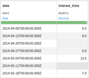
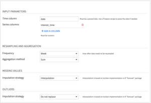
- Time column: Column with date information in parsed date format. If your dates are not parsed, you can use the Parse date processor in a Prepare recipe.
- Series columns: Columns with time series numeric values.
Resampling and aggregation
- Frequency: This determines the amount of time between data points in the cleaned dataset.
- Aggregation method: When multiple rows fall within the same time period, they are aggregated into the cleaned dataset either by summing (default) or averaging their values.
Missing values: Choose one of the following Imputation strategies
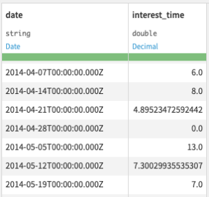
- Interpolate (default) uses linear interpolation for non-seasonal series. For seasonal series, a robust seasonal trend decomposition is used. Linear interpolation is applied to the seasonally adjusted data, and then the seasonal component is added back.
- Replace with average/median/fixed/previous value.
- Do nothing.
Outliers: Choose one of the following Imputation strategies
- Interpolate (default) uses the same technique as for missing values.
- Replace with average/median/fixed/previous value.
- Do nothing.
Outliers are detected by fitting a simple seasonal trend decomposition model using the tsclean method from the forecast package.
1. Train and evaluate forecasting models
Train forecasting models and evaluate their performance on historical data
Input
- Historical dataset: the output of the Clean time series recipe if your time series needs resampling and/or has missing values
Output
- Trained model folder: Folder to save trained forecasting models
- Performance metrics dataset: Performance metrics of forecasting models evaluated on a split of the historical dataset. This dataset will contain the following columns:
- model: the model name
- performance metrics: mean_error, root_mean_square_error, mean_absolute_error, mean_percentage_error, mean_absolute_percentage_error (in percentage), run_time (in seconds)
- evaluation information: evaluation_horizon, evaluation_period, evaluation_strategy
- training_date: the date when you ran the recipe (in UTC)
Settings
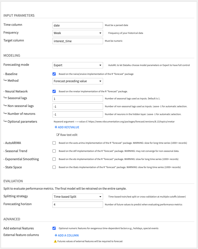
Input parameters
- Time column: Column with date information in parsed date format. If your dates are not parsed, you can use the Parse date processor in a Prepare recipe.
- Frequency: Frequency of your time series
- Target column: The time series you want to predict
Modeling: Choose one of the following Forecast modes
- AutoML (default): Select which models to train and let Dataiku choose parameters among the following models
- Baseline (activated by default)
- Neural Network (activated by default)
- AutoARIMA
- Seasonal Trend
- Exponential Smoothing
- State Space
By default, we only activate two model types: Baseline and Neural Network, as they performed well in our benchmarks. You may select more models, but be aware that some models take more time to compute, or may fail to converge on small datasets. In this case, you will get an error when running the recipe, telling you which model type to deactivate.
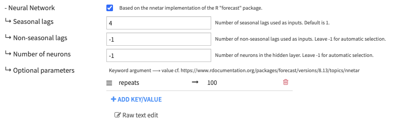
- Expert mode: Gives access to optional parameters that are custom to each model type. For details on each parameter, please refer to the R package documentation.
For instance, if you want to tune the Neural Network model, you can set ↳ Seasonal lags to 4, which corresponds to the P parameter in nnetar. You can set additional model arguments through the ↳ Optional parameters, for instance, repeats ⟶ 100 if you want to ensemble 100 randomly-initialized neural networks together.
Evaluation: Choose one of the following Splitting strategies
- Time-based Split (default): Train/test split where the test set consists of the last H values of the time series.
- You can change H with the Horizon parameter.
- The models will be trained on the train split and evaluated on the test split.
- Time Series Cross-Validation: Split your dataset into multiple rolling train/test splits.
- The models will be retrained and evaluated on their errors for each split. Performance metrics are then averaged across all splits.
- Each split is defined by a cutoff date: the train split is all data before or at the cutoff date, and the test split is the H values after cutoff. H is the Horizon parameter, the same as for the Time-based Split strategy.
- Cutoffs are made at regular intervals according to the Cutoff period parameter, but cannot be before the Initial training parameter.
- Having a large enough Initial training set guarantees that the models trained on the first splits have enough data to converge. You may want to increase that parameter if you encounter model convergence errors.
- The exact method used for cross-validation is described in the Prophet documentation. You can read this article from Rob Hyndman to understand an alternative, simpler implementation.
- Note that Cross-Validation takes more time to compute since it involves multiple retraining and evaluation of models. In contrast, the Time-based Split strategy only requires one retraining and evaluation.
- In order to alleviate that problem, we implemented retraining so that models are refit to each training split but hyperparameters are not re-estimated. This is done on purpose to accelerate computation.
Advanced
- External features (optional): Columns with exogenous numeric regressors that you know in advance, e.g., holidays or special events
- Be careful that future values of these regressors will be required when forecasting (next recipe).
- Only Neural Network and AutoARIMA models can use exogenous regressors.
2. Forecast future values and get historical residuals
Use trained forecasting models to predict future values and/or get historical residuals
Input
- Trained model folder: Folder containing models saved by the “Train and evaluate forecasting models” recipe
- Performance metrics dataset: Dataset with performance metrics computed by the “Train and evaluate forecasting models” recipe
- Optional – Dataset with future values of external features: Only required if you specified external features in the “Train and evaluate forecasting models” recipe
Output
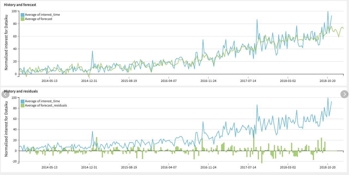
- Forecast dataset: Dataset with predicted future values and/or historical residuals
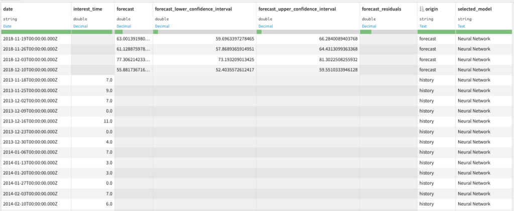
You can use this dataset to build charts and visually inspect the forecast results.
Settings
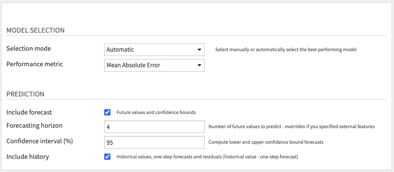
Model Selection: Choose how to select the model used for prediction:
- Automatic: if you want to select the best model according to a specific Performance metric.
- Manual: if you want to select the model yourself.
If you run the “Train and evaluate forecasting models” recipe multiple times, this step selects models within the most recent training session.
Prediction: Choose whether you want to Include forecast, Include history, or both.
If you include the forecast, you can specify the Forecasting Horizon and the probability percentage for the Confidence interval.
If you are including the history, note that forecast residuals are based on one-step forecasts, which are computed AFTER model training on the entire sample. Thus, the columns “forecast” and “forecast_residuals” within the history (cf. “origin” column) should NOT be used to measure model performance. These columns are only included for anomaly detection and feature engineering purposes.
Advanced usage
Forecasts by entity a.k.a. partitioned forecasts
If you want to run the recipes to get one forecast for each entity (e.g. for each product or store), you will need partitioning. That requires having all datasets partitioned by one (only) dimension for the category, using the discrete dimension feature in Dataiku. If the input data is not partitioned, you can use a Sync recipe to repartition it, as explained in this article.